Read microscopy images to numpy arrays with python-bioformats

The python-bioformats library lets you seamlessly read microscopy images into numpy arrays from pretty much any file format.

I recently explained how to use Fiji's Jython interpreter to open BioFormats images, do some processing, and save the result to a standard format such as TIFF. Since then, the CellProfiler team has released an incredible tool, the python-bioformats library. It uses the Java Native Interface (JNI) to access the Java BioFormats library and give you back a numpy array within Python. In other words, it's magic.

Some of the stuff I was doing in the Jython interpreter was not going to fly for a 400GB image file produced by Leica (namely, setting the flag setOpenAllSeries(True)). This file contained 3D images of multiple zebrafish embryos, obtained every 30 minutes for three days. I needed to process each image sequentially.

The first problem was that even reading the metadata from the file resulted in a Java out-of-memory error! With the help of Lee Kamentsky, one of the creators of python-bioformats, I figured out that Java allocates a maximum memory footprint of just 256MB. With the raw metadata string occupying 27MB, this was not enough to contain the full structure of the parsed metadata tree. The solution was simply to set a much larger maximum memory allocation to the JVM.

Once that was done, it was straightforward enough to get an XML string of metadata to get information about all the images contained in the file:

md = bf.get_omexml_metadata('Long time Gfap 260314.lif')

This was my first experience with XML, and I found the official schema extremely intimidating. Thankfully, as usual, Python makes common things easy, and parsing XML is a very common thing. Using the xml package from the Python standard library, it is easy enough to get the information I want from the XML string:

from xml.etree import ElementTree as ETree
mdroot = ETree.fromstring(md)

You might have gathered that the ElementTree object contains a rooted tree with all the information about our file. Each node has a tag, attributes, and children. The root contains information about each series:

('{http://www.openmicroscopy.org/Schemas/OME/2011-06}Image', {'ID': 'Image:121', 'Name': '41h to 47.5 hpSCI/Pos021_S001'})

And each series contains information about its acquisition, physical measurements, and pixel measurements:

>>> for a in mdroot[300]:
...     print((a.tag, a.attrib))
...
('{http://www.openmicroscopy.org/Schemas/OME/2011-06}AcquiredDate', {}),
('{http://www.openmicroscopy.org/Schemas/OME/2011-06}InstrumentRef', {'ID': 'Instrument:121'}),
('{http://www.openmicroscopy.org/Schemas/OME/2011-06}ObjectiveSettings', {'RefractiveIndex': '1.33', 'ID': 'Objective:121:0'}),
('{http://www.openmicroscopy.org/Schemas/OME/2011-06}Pixels', {'SizeT': '14', 'DimensionOrder': 'XYCZT', 'PhysicalSizeY': '0.445197265625', 'PhysicalSizeX': '0.445197265625', 'PhysicalSizeZ': '1.9912714979001302', 'SizeX': '1024', 'SizeY': '1024', 'SizeZ': '108', 'SizeC': '2', 'Type': 'uint8', 'ID': 'Pixels:121'})

I only need a fraction of this metadata, so I wrote a function, parse_xml_metadata, to parse out the image names, their size in pixels, and their physical resolution.

Armed with this knowledge, it is then straightforward to preallocate a numpy array for each image and read the image from disk:

from matplotlib import pyplot as plt, cm
from lesion.lifio import parse_xml_metadata
import numpy as np
from __future__ import division

filename = 'Long time Gfap 260314.lif'
rdr = bf.ImageReader(filename, perform_init=True)
names, sizes, resolutions = parse_xml_metadata(md)
idx = 50 # arbitrary series for demonstration
size = sizes[idx]
nt, nz = size[:2]
image5d = np.empty(size, np.uint8)
for t in range(nt):
    for z in range(nz):
        image5d[t, z] = rdr.read(z=z, t=t, series=idx, rescale=False)
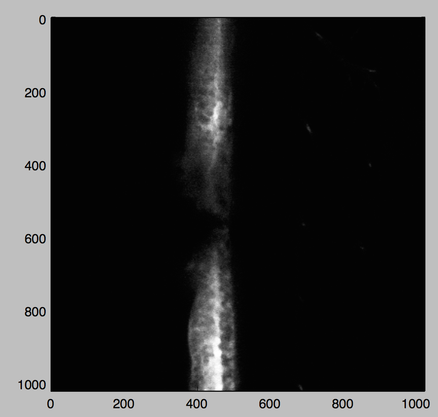
plt.imshow(image5d[nt//2, nz//2, :, :, 0], cmap=cm.gray)
plt.show()

Boom. Using Python BioFormats, I've read in a small(ish) part of a quasi-terabyte image file into a numpy array, ready for further processing.

Note: the dimension order here is time, z, y, x, channel, or TZYXC, which I think is the most efficient way to read these files in. My wrapper allows arbitrary dimension order, so it'll be good to use it to figure out the fastest way to iterate through the volume.

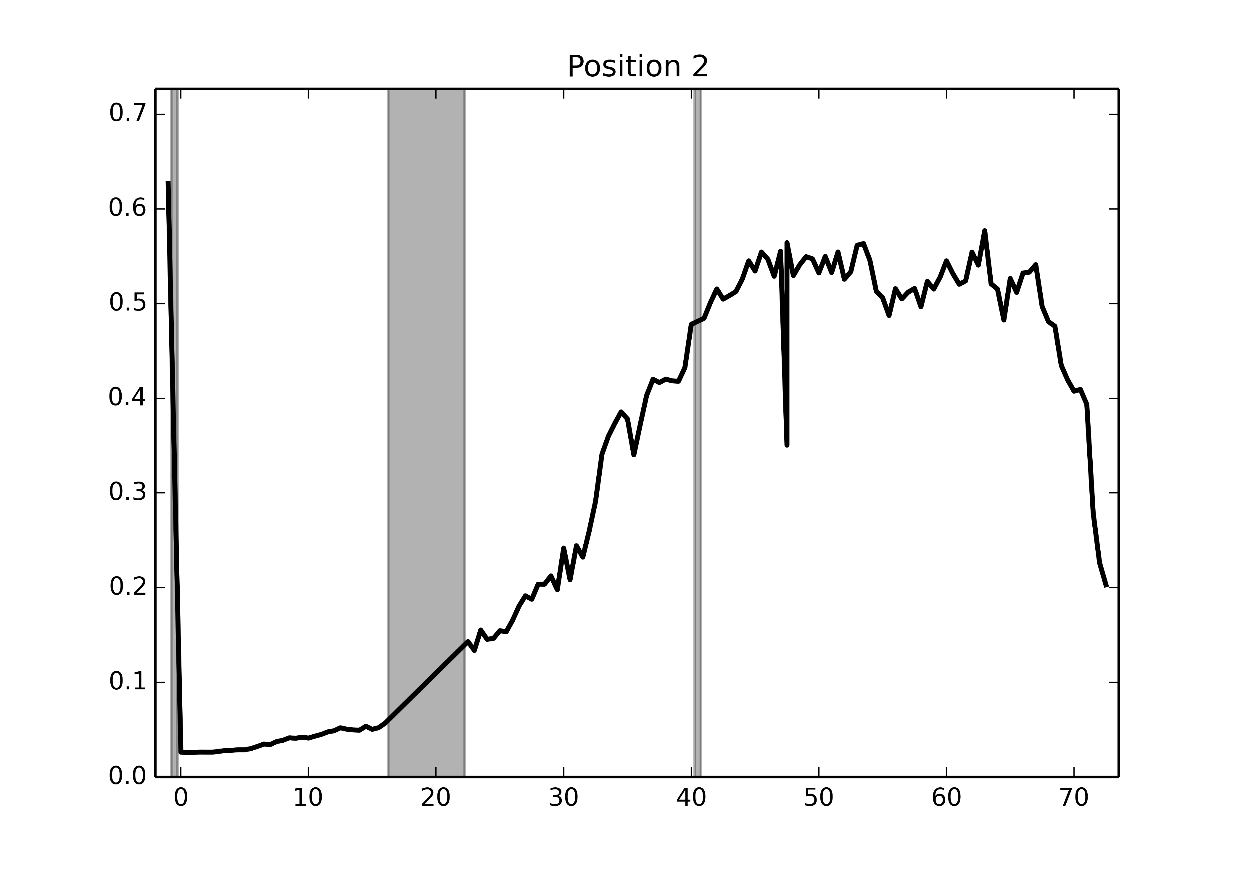
In my case, I'm looking to extract statistics using scikit-image's profile_line function, and plot their evolution over time. Here's the min/max intensity profile along the embryo for a sample stack:

I still need to clean up the code, in particular to detect bad images (no prizes for guessing which timepoint was bad here), but my point for now is that, thanks to Python BioFormats, doing your entire bioimage analysis in Python just got a heck of a lot easier.